Checking access…

Built on Google Cloud
Omni Pinpoint

Location
Intelligence

High-resolution location intelligence derived from network mobility signals — delivering crowd movement analytics, origin-destination flows, venue attribution, and dwell-time scoring for urban planning, retail intelligence, and public safety applications. Built on a scalable GCP spatial pipeline with 100m – 300m precision.

Sub-300m H3 Precision Crowd Movement Analytics Origin-Destination Flows Venue & Gate Intelligence BQ Spatial + Geo Dataflow
Omni Pinpoint — Location Intelligence
Product Overview

Location Intelligence Capabilities

Omni Pinpoint transforms raw network mobility signals into a full-stack geospatial intelligence platform. Eight analytical modules — from population density heatmaps and origin-destination flow modelling through to AI-driven spatial querying — share a single BigQuery spatial pipeline and deliver insights at sub-300m H3 resolution across any geography.

Platform Modules — 8 Analytics Views
🌡️
Population Heatmap
Real-time crowd density and mobility heat signatures rendered at H3 resolution across any defined geography. Identifies high-traffic zones, congestion clusters, and temporal demand peaks.
Density · H3 Spatial
🔀
OD Flows — Day Level
Full origin-destination matrices aggregated at the daily level. Shows where people travel from and to across zones, supporting strategic transport planning and demand forecasting.
OD Matrix · Daily
⏱️
OD Flows — Hour Level
The same origin-destination analysis broken down by hour — enabling operators to observe how flow patterns shift through morning peaks, midday, evening surges, and overnight. Time-slider playback across any date.
OD Matrix · Hourly
🏛️
Gate & Venue Utilisation
Entry and exit counts, dwell durations, and flow rankings for every defined access point or venue. Ranks corridors by volume, highlights bottlenecks, and surfaces demographic composition per gate.
Venue Intel · Capacity
🚪
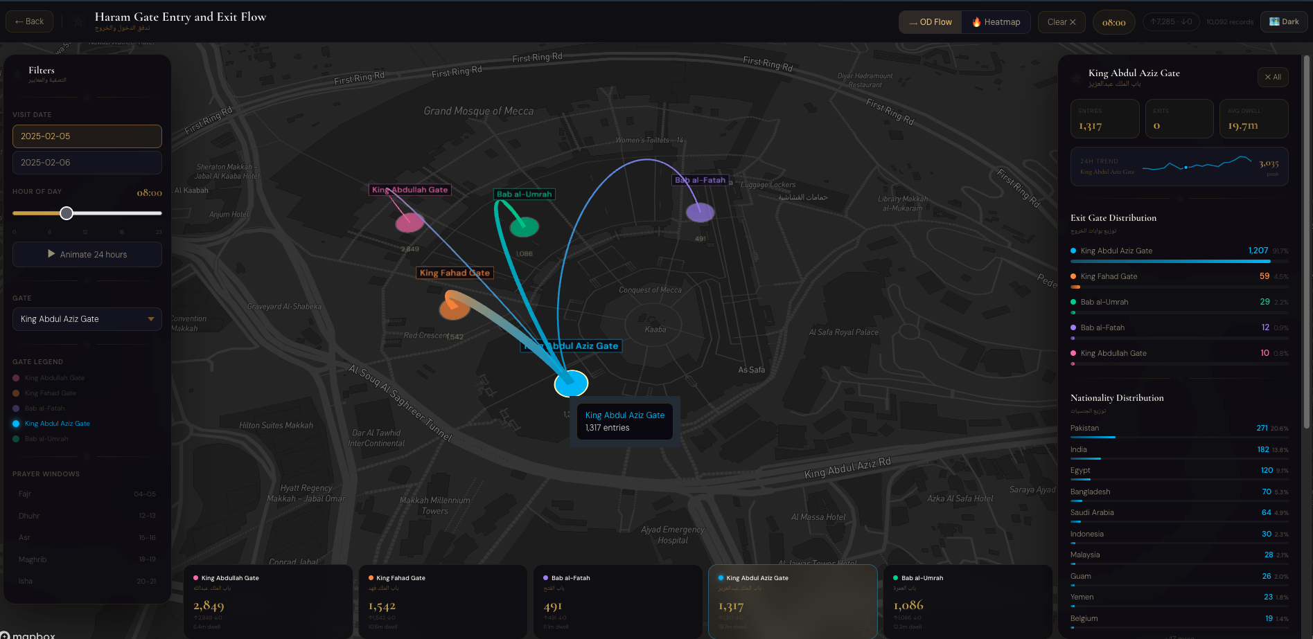
Entry-Exit Flow Monitoring
Arc-based visualisation of crowd flows between entry and exit zones in real time. Each arc scales by movement volume and is colour-coded by direction, with per-zone ingress/egress KPIs and demographic breakdowns on the side panel.
Flow Arcs · Real-time
🛤️
Individual Route Traces
Path-level movement traces reconstructed from network signals at H3 resolution. Reveals route preference distributions, identifies underutilised paths, and supports network demand modelling for new infrastructure.
Path Intel · H3 Routes
🛣️
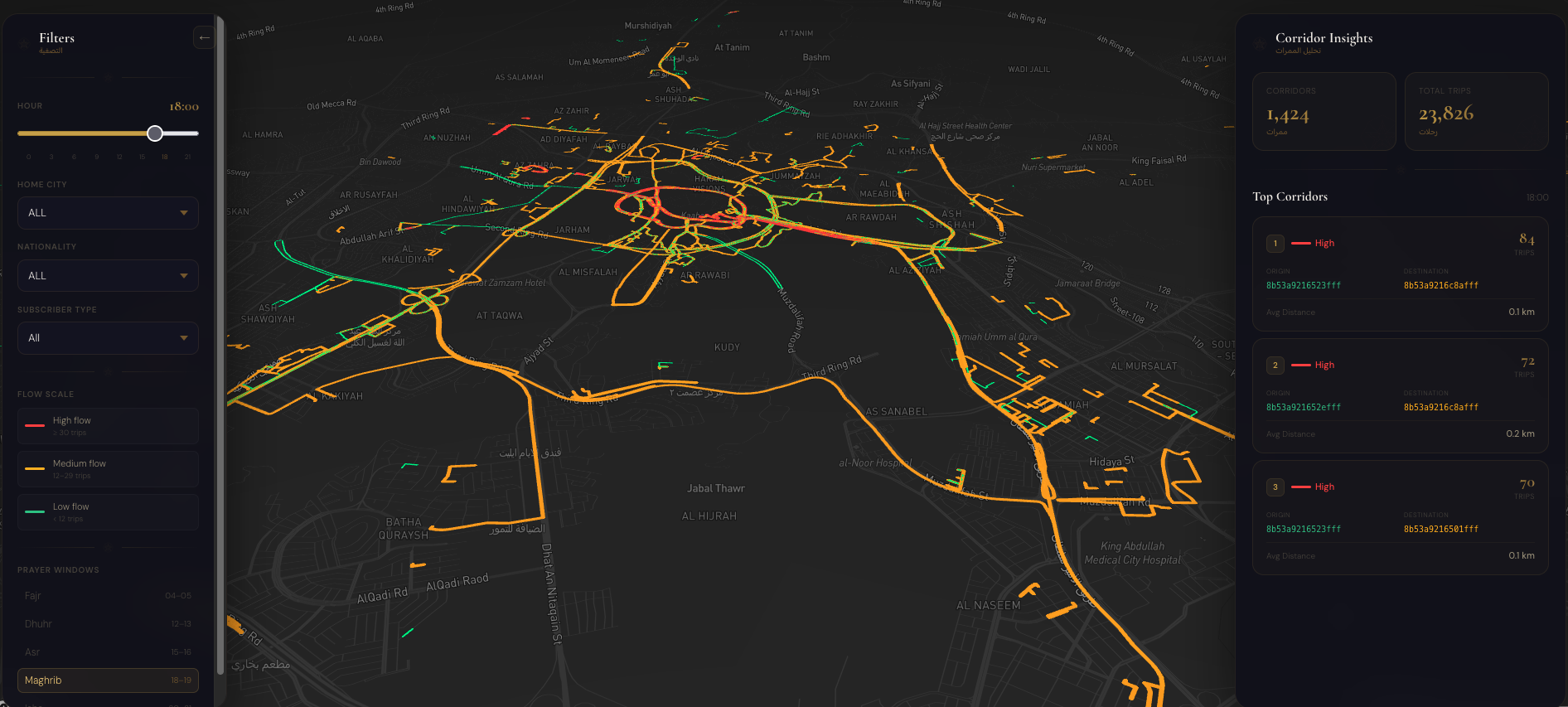
Road Movement & Corridors
The road network rendered as a live movement heatmap — corridors coloured from green (free flow) to red (high congestion). Ranked top corridors, unique device counts, and hourly time-slider playback for any date range.
Road Network · Corridors
🤖
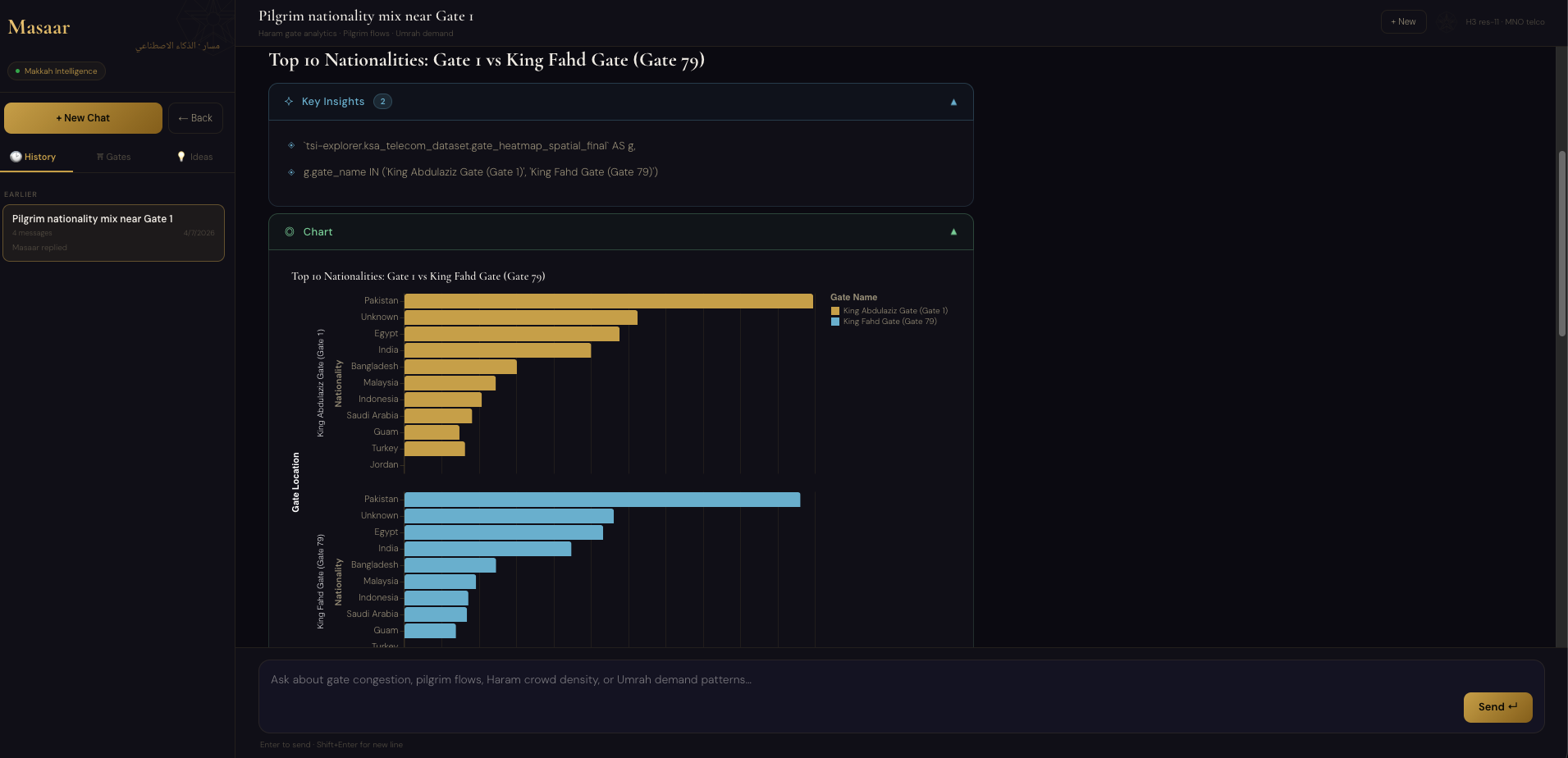
Masaar AI Agent
Conversational AI copilot layered directly over all spatial data. Analysts ask natural language questions — the agent surfaces ranked insights, cross-zone comparison charts, and narrative summaries without any SQL expertise required.
AI Copilot · NL Queries
Live Dashboard Screenshots
🏛️
Module 01
Zone Entry & Exit Flow Monitoring
Entry-Exit Flow Monitoring
What it shows
Real-time arc visualisation of crowd flows between defined entry and exit zones. Each arc represents aggregated movement volume between two points, scaled by traffic intensity and colour-coded by flow direction.
Key Metrics
Per-zone ingress and egress counts · Dwell duration distribution · Demographic composition breakdown · Hourly temporal filters to isolate peak demand windows.
Use Cases
Venue capacity planning · Access control optimisation · Event crowd management · Infrastructure demand forecasting for new entry points.
🛣️
Module 02
Road Movement & Corridor Intelligence
Road Movement and Corridor Intelligence
What it shows
The road network rendered as a live movement heatmap — corridors coloured from green (free flow) through amber to red (high congestion) based on subscriber movement density along each route segment.
Key Metrics
Corridor-level movement volumes · Ranked top routes by traffic intensity · Unique device counts and total movement events · Time-slider for hourly playback across any date range.
Use Cases
Transport network planning · Congestion hotspot identification · Route demand modelling for new infrastructure · Real-time traffic pattern monitoring for operations teams.
🤖
Module 03
Masaar AI Insights Agent
What it shows
A conversational AI interface layered directly over the spatial dataset. Analysts type natural language questions — the agent surfaces key insights, comparison charts, and ranked breakdowns drawn live from the underlying BigQuery spatial tables.
Key Capabilities
Natural language spatial queries · Auto-generated charts from query results · Cross-zone comparisons in a single prompt · Demographic and behavioural segment analysis without SQL expertise.
Use Cases
On-demand insight generation for non-technical stakeholders · Rapid ad-hoc comparisons between zones or time periods · Executive-ready summaries derived from real mobility data without manual dashboarding.
Data Requirement

Input Data Specifications

Omni Pinpoint is powered by three datasets: a high-frequency Footfall feed capturing device-level location events, a Master Dataset resolving raw coordinates into a full geographic hierarchy with spatial metadata, and a Demographics feed enabling crowd composition analysis by age, gender, and segment.

📍
Foot Traffic
Daily ingestion · raw location pings
~10 TB/day
Raw daily
10 TB
~35B rows (70M subs)
Monthly raw
~300 TB
~60B pings
Compressed
~3 TB
Parquet · 3.5×
FieldTypeDescription
sub_hashSTRINGPseudonymised subscriber token — join key to Demographics
ping_tsTIMESTAMPLocation observation timestamp (UTC)
latitudeFLOAT64GPS latitude (WGS84, 6 decimal places)
longitudeFLOAT64GPS longitude (WGS84, 6 decimal places)
accuracy_mINT64Radial accuracy estimate in metres (100–300m typical)
cell_idSTRINGServing cell site identifier — used for coverage validation
dwell_minutesINT64Minutes spent at the inferred location before movement
date_partitionDATEPartition key — used for rolling window pruning in BQ
🗺️
Master Dataset
Quarterly refresh · spatial reference
~200 MB static
Static volume
200 MB
Full tile set
H3 resolution
9 – 12
Sub-300m tiles
Refresh
Qtrly
+ ad-hoc patches
FieldTypeDescription
tile_idSTRINGUnique tile identifier — join key to Footfall lat/lon
h3_indexSTRINGH3 hierarchical spatial index at resolution 9–12
countrySTRINGISO 3166-1 alpha-2 country code
countySTRINGAdministrative county or equivalent region
citySTRINGCity or urban area name
districtSTRINGSub-city district or neighbourhood
poi_typeSTRINGPoint-of-interest category: retail · transit · leisure · health
geofence_wktGEOGRAPHYWKT polygon for the tile boundary — used in BQ spatial joins
centroid_latFLOAT64Tile centroid latitude (WGS84)
centroid_lonFLOAT64Tile centroid longitude (WGS84)
👥
Demographics
Monthly snapshot · subscriber attributes
~2 TB/month
Monthly volume
~2 TB
Full base
Refresh
Monthly
Snapshot + delta
Privacy
k-anon
Pseudonymised
FieldTypeDescription
sub_hashSTRINGJoin key — same pseudonymised token as Foot Traffic
age_bandSTRINGAge cohort bracket (e.g. 18–24, 25–34, 35–44 …)
genderSTRINGInferred or declared gender classification
segmentSTRINGBehavioural segment label (urban commuter, suburban family …)
nationalitySTRINGISO country code of subscriber nationality
tenure_bandSTRINGLength of relationship: <1yr · 1–3yr · 3–5yr · 5yr+
home_regionSTRINGInferred home region from overnight dwell pattern
snapshot_monthDATEPartition key — month the snapshot was generated

Processing Pipeline

Footfall events are spatially joined against the Master Dataset in BigQuery to resolve raw coordinates into place-aware records, then enriched with demographic attributes before writing to the spatial output tables delivered via Analytics Hub.

📍
Foot Traffic
10 TB/day
›
🗺️
Master Join
BQ spatial
›
👥
Demo Enrich
sub_hash join
›
🔄
Geo Dataflow
Dwell · POI
›
📡
Analytics Hub
Client delivery
Cost Estimates · Jul 2026 → Dec 2030

Processing & Storage · BQ Flex Slots

Omni Pinpoint processes 10 TB/day of raw location pings from 70M subscribers (~500 rows/sub/day, ~35B rows/day total), spatial-joins with the 200 MB Master Dataset and 4M-row Demographics table, then aggregates to 1.2M POI-level hourly and daily summary tables. Hourly tables use a configurable rolling window; daily tables retain 12 months. The dominant cost is daily batch compute on BigQuery Flex Slots — storage is secondary.

Daily Compute
$120
500 slots · 6 hrs
Monthly Compute
$3,600
BQ Flex Slots
Annual Compute
$43,800
2026 baseline
Agg Storage (SS)
~969 GB
Hourly 3mo + daily 12mo

5-Year Annual Cost Forecast ($K) — Compute + Storage

BQ Flex Slots compute (gold) stacked with storage cost (teal) · 18% YoY growth · compute:storage ~195:1 at baseline

5-Year Grand Total
—
BQ Flex Slot CUDs save 20% (annual) or 40% (3-year). Applied to compute only — storage already at long-term $0.01/GB/mo.
0%10%20%30%40%

Stage 1 — Platform Selection & Daily Processing Pipeline

BigQuery Flex Slots is the recommended platform: a single daily SQL + GEO batch job with no persistent compute, no Spark overhead, and native H3 spatial support. On-demand BQ pricing at $6.25/TB would cost ~$62/day just for the raw 10 TB scan alone — Flex Slots burst capacity eliminates per-query billing entirely during the daily window.

⚡
BigQuery Flex Slots · $0.04/slot/hr · Zero idle cost

Burst capacity activated only during the 6-hour daily processing window. At 35B rows/day, H3 coordinate conversion is a compute-heavy UDF pass on every ping, and the 70M-subscriber demographic join is a large shuffle — together requiring a minimum of 500 slots for nightly completion. sub_hash is the pseudonymised join key across all three input datasets. Native BQ GEO functions and H3 extensions handle all spatial operations — no external Spark cluster needed. The 200 MB Master Dataset is broadcast-joined, making the spatial lookup step highly efficient.

Flex Slots · $0.04/slot/hr Zero idle cost BQ GEO + H3 native 6-hr daily window No infra management
5-Step Daily Pipeline — 35B rows in · 1.2M POI aggregates out
📍
1. Scan
10 TB raw pings
35B rows · 70M subs
›
🗺️
2. Spatial Join
H3 → POI lookup
200 MB Master Dataset
›
👥
3. Demo Enrich
sub_hash → attrs
age · gender · seg · nat
›
⏱️
4. Hourly Agg
POI × hr × demo
~461M rows/day
›
📅
5. Daily Agg
POI × day × demo
~19M rows/day

Stage 2 — Compute · BQ Flex Slots · Interactive Model

Slot count × daily window × $0.04/slot/hr determines the full compute cost. At 35B rows/day, the H3 coordinate-to-hexagon conversion (a compute-intensive UDF operation on every ping) combined with the 70M-subscriber demographic shuffle-join makes 500 slots the practical minimum for a 6-hour nightly window. At 200 slots the same pipeline requires 12–15 hours — incompatible with a daily cadence. Cost scales linearly — halving slots roughly doubles the required window, keeping daily cost identical.

Compute Parameters
Burst slot count during the daily processing window. 500 slots is the practical minimum for 35B rows/day: H3 coordinate conversion (compute-heavy UDF on every ping) + 70M-sub demographic shuffle-join + two aggregation steps complete within 6 hours. At 200 slots the pipeline would take 12–15 hours.
Hours the Flex Slot reservation is active per day. Cost = slots × hours × $0.04. 6 hours gives comfortable headroom for the 35B-row spatial and demographic join pipeline.
YoY growth in subscriber base and raw data volume — drives both compute and storage scaling in the 5-year forecast.
Daily pipeline cost · 2026
$120 /day
Slots500
Window6 hrs
Flex rate$0.04/slot/hr
Daily cost$120
Monthly$3,600
Annual$43,800
Agg Storage — steady-state
Hourly (rolling SS)~829 GB
Daily (12-mo SS)~140 GB
Storage cost: ~$224/yr · BQ Active $0.020 · Dormant $0.010/GB/mo
Compute dominates total cost.

Stage 3 — Aggregated Output Storage · Rolling Windows

Each day produces ~9.2 GB of hourly aggregation output (1.2M POIs × 24 hrs × 16 demo dims) and ~384 MB of daily rollup. Both tables use rolling partition expiry — old days auto-delete as new ones arrive. BQ's blended active/long-term pricing brings total aggregated storage to ~$224/year at the default ~969 GB steady-state — under 0.6% of the annual compute cost at 500 slots.

Storage Parameters
Network target is 1.2M POIs — primary driver of aggregation output row count.
Unique demo combos per POI-hour cell (e.g. 4 age × 2 gender × 2 nationality = 16).
Hourly tables are large (~9 GB/day). 3-month rolling window is recommended. Daily tables always retain 12 months.
Storage Breakdown · Steady State
Hourly SS
829 GB
3-month rolling
Daily SS
140 GB
12-month rolling
Annual Cost
$224
Active $0.020 · Dormant $0.010/GB/mo
TableRows/dayGB/dayActive (≤6mo)Dormant (>6mo)$/yr
Hourly (POI×hr×demo)461M9.2 GB829 GB—$199
Daily (POI×day×demo)19M0.4 GB69 GB71 GB$25
Total—9.6 GB898 GB71 GB$224

5-Year Cost Forecast 2026–2030 · Detailed Breakdown

Annual compute scales with subscriber volume growth at the configured rate. Storage grows proportionally with data volume. Storage cost remains under 1% of the total throughout the forecast period — this is a compute-dominated model.

YearDaily ComputeAnnual ComputeHourly SS (GB)Daily SS (GB)Storage Cost / yrTotal
5-Yr Total · Yr 5 SS↑——————
Cost summary: At 500 slots × 6 hrs/day — the minimum reliable allocation for 35B rows of H3 spatial processing + 70M-sub demographic joins — compute costs $120/day = $43,800/year. Storage at 1.2M POIs (hourly 3-month + daily 12-month rolling) totals ~969 GB steady-state — priced as BQ Active ($0.020/GB/mo) for the most recent 6 months and Dormant ($0.010/GB/mo) for prior months — ≈$224/year. The compute:storage ratio is ~195:1. At 200 slots the pipeline would overrun the nightly window (12–15 hours) and risk job failure on memory pressure. Adjust the slot slider and hourly retention window to model alternatives; apply the CUD slider to see the impact of GCP committed-use agreements.

Platform Summary

📄 View Full Summary

Plain-English guide to all cost models, assumptions, strategies, and caveats across every product page.